Let’s assume that we want to analyze a wide range of products that regularly generate revenues (for a company like Gühring, a mid-sized manufacturer of rotary cutting tools, that number easily exceeds 8,000!). The objective of an early-warning system is to identify when something starts to go astray. First, we have to define exactly what we mean by that.

Sales revenues are atypical when they:

1. Vary considerably over the past six months
2. Increase greatly
3. Drop drastically
4. Increase greatly and then drop drastically
5. Perform differently than the total trend

Points 1 through 4 basically translate into the statistical spread of a time-series’ values around the mean of the respective time series. For point 5 we also need comparative or reference data.

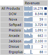
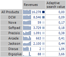
Let’s use the left table below as an example. It shows the revenue development of individual products over the past six months. The values are not sorted. Compare this table with the one on the right. This table sorts the products so that those with a revenue development similar to that of all products are displayed at the top.

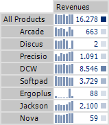
Our task today is to automate this sorting. In order to do this, we first need to determine the statistical spread of each product’s revenues compared to total revenues (i.e. all products). Large variances suggest a very different development, while small variances indicate a similar development pattern.

Since the revenues for each product are very different (signalized by the cell coloring to the right of the table), we cannot compare the revenue values directly. In order to make the revenue development of all products comparable, we will first have to calculate the mean over the past six months for each product so we can use this number as the normed value per product:

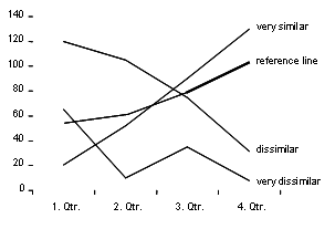
To do this, we simply divide the period values of a product by the individual product mean. This allows us to compare the revenue development of all products. In addition, we can calculate the normed development for total revenues and use this as a reference line:

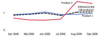
However, we don’t just want to analyze the different revenue developments using a chart. We want to calculate the difference using a KPI. As a result, we will determine the standard variance for each product based on the reference line. This means that we will display the difference between the normed and individual period values per product and month (in this case, April through September):

Difference (Month X) = Normed Revenues (Product) – Normed Revenues (Reference Line)

To eliminate discrepancies in signs, we will square the differences per month and then add up the squared difference values per product. When we then take the square root of the sum, we have calculated a KPI that I like to call an “adaptive search value”. With the help of this KPI, we can automatically search our table for typical and atypical revenue developments. We can also use this search value to sort the table from “similar” to “very different”:

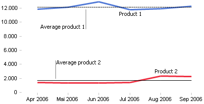
The optical comparison of the time series with the time series for “all products” shows that our KPI is very reliable in calculating similarities. Since this benchmark automatically adapts to the underlying data, it also delivers trustworthy conclusions for a completely different total revenue development.